あの木に花が咲く時、きっとAIも自然を愛でる

AIって結局何なのかよく分からないので、とりあえず100日間勉強してみた Day13

経緯についてはこちらをご参照ください。

AIって結局何なのかよく分からないので、とりあえず100日間勉強してみた Day0

■本日の進捗

●決定木モデルを使ってみる

■はじめに

今回は回帰にもクラス分類にも適用可能な決定木モデルを使っていきたいと思います。

■決定木

決定木はデータをある条件で再帰的に分割して、入力データを分類していく階層を構築するアルゴリズムです。

データセットの最上位である「根（Root Node）」から分岐が始まり、「内部ノード（Internal Nodes）」を通じて「葉（Leaf Nodes）」に予測結果を割り当てます。

このことから、（浅い階層であれば）モデルを理解しやすく、前処理の必要もないのが特徴です。早速、あやめデータセットに適用してみたいと思います。

from sklearn.datasets import load_iris
from sklearn.tree import DecisionTreeClassifier, export_graphviz
from sklearn.model_selection import train_test_split

iris = load_iris()
X = iris.data
y = iris.target

X_train, X_test, y_train, y_test = train_test_split(X, y, test_size=0.3, random_state=8)

model = DecisionTreeClassifier(max_depth=3)
model.fit(X_train, y_train)

dot_data = export_graphviz(model, out_file="decisionTree_iris_viz.dot", 
                           feature_names=iris.feature_names,  
                           class_names=iris.target_names,  
                           filled=True, rounded=True,  
                           special_characters=True)

print("train score: {}".format(model.score(X_train, y_train)))
print("test score: {}".format(model.score(X_test, y_test)))

train score: 0.9904761904761905
test score: 0.8888888888888888

複雑さの制御のために「事前枝刈り」として成長率を最大3にして学習させました。これでも過剰適合のように見えますが、スコアはとても高いです。
ちなみにこのモデルは解釈のために可視化することが容易で、機械学習に触れたことのない人にも大変理解しやすい形で可視化できます。

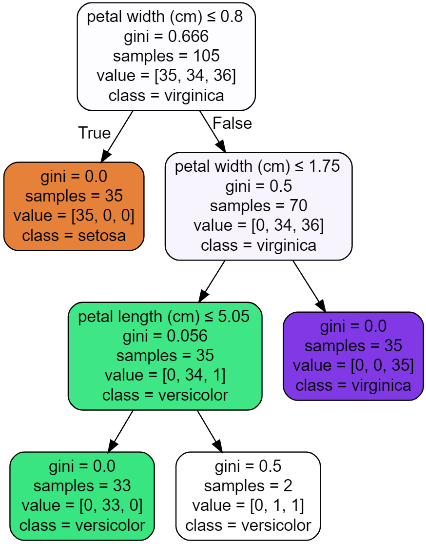
それぞれの条件分岐においてTrueかFalseかで分岐していき、最終的に行き着いた葉がそのデータにおけるクラスに分類されます。（もちろん同様に回帰も可能）

また、学習に用いた特徴量をmodel.feature_importances_という変数に重要度という数値で格納されているので、これを参照することでどの特徴量をどれだけ用いたのかを可視化することも可能です。

from sklearn.datasets import load_iris
from sklearn.tree import DecisionTreeClassifier, export_graphviz
from sklearn.model_selection import train_test_split
import matplotlib.pyplot as plt
import numpy as np

iris = load_iris()
X = iris.data
y = iris.target

X_train, X_test, y_train, y_test = train_test_split(X, y, test_size=0.3, random_state=8)

model = DecisionTreeClassifier(max_depth=3)
model.fit(X_train, y_train)

feature_importances = model.feature_importances_
features = iris.feature_names

plt.figure(figsize=(8, 6))
plt.barh(np.arange(len(features)), feature_importances, align='center')
plt.yticks(np.arange(len(features)), features)
plt.xlabel('Feature Importance')
plt.ylabel('Features')
plt.title('Feature Importance of Iris Decision Tree')
plt.show()

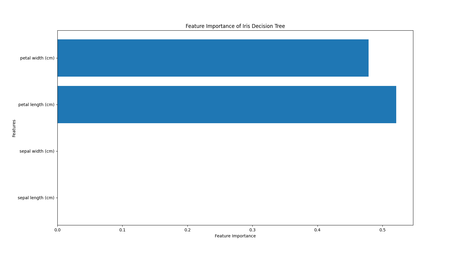
このモデルは花弁のデータのみを使ってモデルを作成していることが分かります。ここでガクのデータが相関がなかったり重要な情報ではないという意味ではないことに注意してください。あくまで「今回の学習においては重要じゃなかった」だけで、パラメータをいじってモデルを再構築すれば全く違った特徴量の構成になることもあり得ます。少なくとも花弁の幅と長さの2つの特徴量にはクラスを分類するために重要な情報が含まれていた、というだけです。また、「花弁が長いならどの品種なのか」ということもこれでは分かりません。

■ランダムフォレスト

決定木は単純で理解もしやすくデフォルトの設定で簡単に高いスコアのモデルを学習できるものの、過剰適合しやすいという側面も持っています。（先ほども事前枝刈りで深さ3までという制約を入れたのにも関わらず過剰適合していました。）

これを解消するべく決定木をベースにした様々なアンサンブル学習アルゴリズムが開発されていて、ランダムフォレストはその一種です。

ランダムフォレストとは、その名の通りランダムな方向に過剰適合した決定木モデルをたくさん作り、その結果の平均を取れば過剰適合の度合いを減らせるという考え方で構築されたアルゴリズムです。まさに木がたくさんあるから森。素晴らしいネーミングだと思います。早速あやめデータセットに適用してみます。今回作る決定木の数は3本です。

import numpy as np
import matplotlib.pyplot as plt
from sklearn.datasets import load_iris
from sklearn.model_selection import train_test_split
from sklearn.ensemble import RandomForestClassifier
from itertools import combinations

data = load_iris()
X = data.data
y = data.target

X_train, X_test, y_train, y_test = train_test_split(X, y, test_size=0.3, random_state=8)

n = 3
model = RandomForestClassifier(n_estimators=n, max_depth=3, random_state=8)
model.fit(X_train, y_train)

print("train score: {}".format(model.score(X_train, y_train)))
print("test score: {}".format(model.score(X_test, y_test)))

train score: 0.9714285714285714
test score: 0.8888888888888888

決定木を3つしか作っていないので森そのものですね（）
先ほどの決定木とほとんど同じパラメータですが、テストスコアをそのままにトレーニングスコアが少し下がりました。明らかな過剰適合を改善することが目的だったので良い兆候かもしれません。

このパラメータにおける決定境界を可視化することもできますが、最終的な学習モデルとは違い、個々の特徴量の組み合わせごとに学習しなおした決定境界であることに注意してください。これは4つの特徴量で学習したモデルの決定境界を見るには2次元プロットでは厳しいためですが、各組み合わせでの決定境界でもランダムフォレストの挙動は理解できると思います。

import numpy as np
import matplotlib.pyplot as plt
from sklearn.datasets import load_iris
from sklearn.model_selection import train_test_split
from sklearn.ensemble import RandomForestClassifier
from itertools import combinations

data = load_iris()
X = data.data
y = data.target

feature_combinations = list(combinations(range(X.shape[1]), 2))

plt.figure(figsize=(15, 10))

for i, (f1, f2) in enumerate(feature_combinations):
    plt.subplot(2, 3, i + 1)
    
    X_train, X_test, y_train, y_test = train_test_split(X[:, [f1, f2]], y, test_size=0.3, random_state=8)

    model = RandomForestClassifier(n_estimators=3, max_depth=3, random_state=8)
    model.fit(X_train, y_train)

    x_min, x_max = X[:, f1].min() - 1, X[:, f1].max() + 1
    y_min, y_max = X[:, f2].min() - 1, X[:, f2].max() + 1
    xx, yy = np.meshgrid(np.arange(x_min, x_max, 0.01), np.arange(y_min, y_max, 0.01))

    Z = model.predict(np.c_[xx.ravel(), yy.ravel()])
    Z = Z.reshape(xx.shape)

    plt.contourf(xx, yy, Z, alpha=0.3, cmap=plt.cm.coolwarm)
    plt.scatter(X[:, f1], X[:, f2], c=y, edgecolor='k', marker='o', cmap=plt.cm.coolwarm)
    
    plt.xlabel(data.feature_names[f1])
    plt.ylabel(data.feature_names[f2])
    plt.title(f'Decision Boundary using {data.feature_names[f1]} and {data.feature_names[f2]}')

plt.tight_layout()
plt.show()

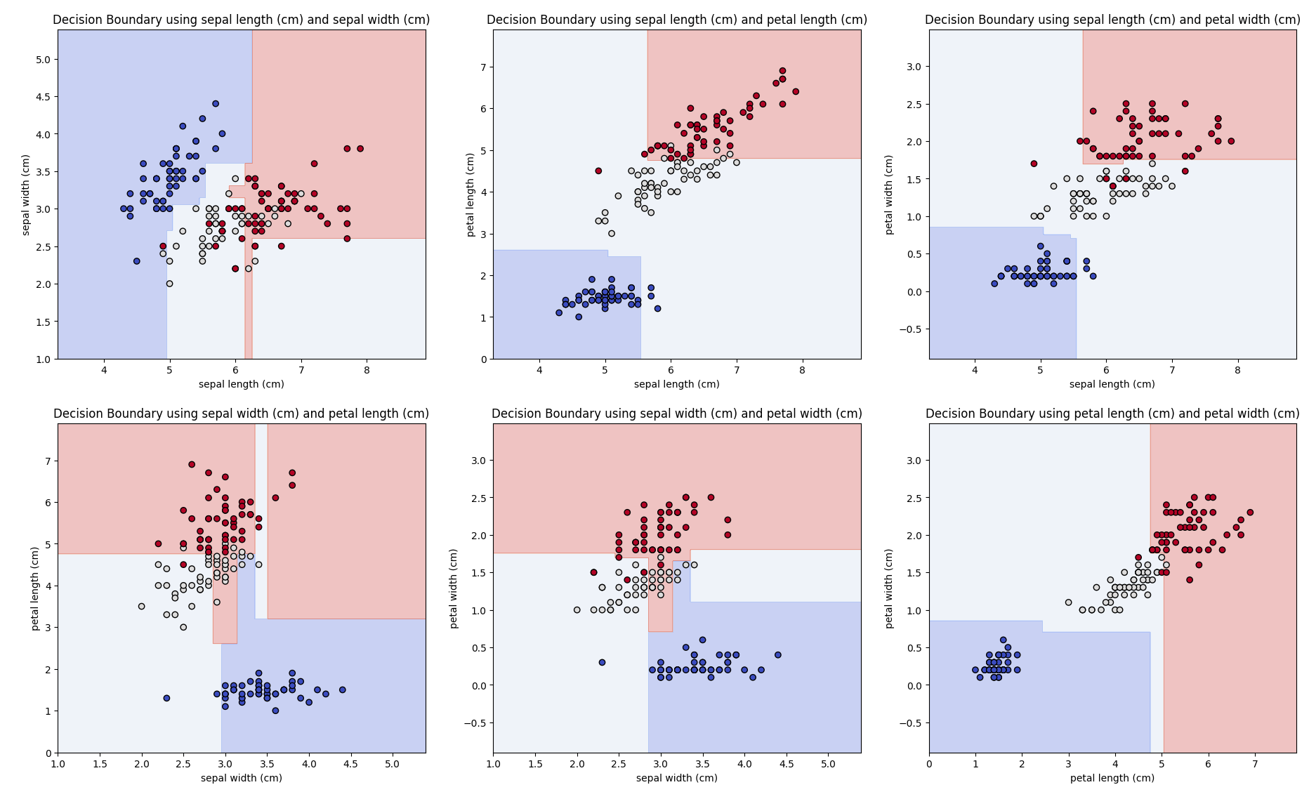
それぞれの特徴量に対してある程度分類できていそうですが、まだまだ粗が目立ちます

また、このランダムフォレストにも欠点があり、計算コストが上がることはもちろん、決定木のメリットであるモデルの理解が難しくなってしまいます。（先ほどの分岐の図が大規模になり何十個、何百個とある様子を想像してみてください。）

ちなみに木の数を10倍（30本、単位合ってる？）にすると下記のように極端な決定境界が減り均したような形になりました。スコア的には更なる過剰適合になったもののテストスコアが大幅に上がりました。

train score: 1.0
test score: 0.9111111111111111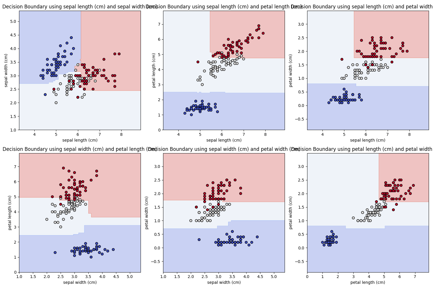

■勾配ブースティング回帰木

勾配ブースティング回帰木（GBDT）はブースティングという複数の簡単な決定木（弱学習機：weak learner）を組み合わせて、より強力なモデルを作ります。回帰という名前ですが、これもクラス分類にも適用可能です。1つ前の決定木の誤分類を次の決定木で修正するように構築し直すことで逐次学習していきます。

ランダムフォレストとは違い乱数性はないですが、弱学習機（簡単なモデル）を作るので予測速度的なメリットもあるのが特徴です。新たなパラメータとして学習率（learning rate）があり、次の決定木にどれだけ影響を与えるかを調節できます。

同様にあやめデータセットに適用してみます。

import numpy as np
import matplotlib.pyplot as plt
from sklearn.datasets import load_iris
from sklearn.model_selection import train_test_split
from sklearn.ensemble import GradientBoostingClassifier

data = load_iris()
X = data.data
y = data.target

X_train, X_test, y_train, y_test = train_test_split(X, y, test_size=0.3, random_state=8)

n = 100
model = GradientBoostingClassifier(n_estimators=n, learning_rate=0.1, max_depth=3, random_state=8)
model.fit(X_train, y_train)

print("train score: {}".format(model.score(X_train, y_train)))
print("test score: {}".format(model.score(X_test, y_test)))

train score: 1.0
test score: 0.8888888888888888

学習率0.1で100本の決定木をこれまでと同じ深さで学習させてみましたが、スコアはこれまでと同じ程度でした。

ここからいくつかのパラメータを振って最適化してみたいと思います。

import numpy as np
import matplotlib.pyplot as plt
from sklearn.datasets import load_iris
from sklearn.model_selection import train_test_split
from sklearn.ensemble import GradientBoostingClassifier

data = load_iris()
X = data.data
y = data.target

X_train, X_test, y_train, y_test = train_test_split(X, y, test_size=0.3, random_state=8)

train_scores = []
test_scores = []
depth_range = range(1, 11)

for depth in depth_range:
    model = GradientBoostingClassifier(n_estimators=100, learning_rate=0.1, max_depth=depth, random_state=8)
    model.fit(X_train, y_train)
    
    train_scores.append(model.score(X_train, y_train))
    test_scores.append(model.score(X_test, y_test))

plt.plot(depth_range, train_scores, label='Train Score', marker='o')
plt.plot(depth_range, test_scores, label='Test Score', marker='o')
plt.xlabel('max_depth')
plt.ylabel('Score')
plt.title('Train and Test Scores vs max_depth')
plt.legend()
plt.grid(True)
plt.show()

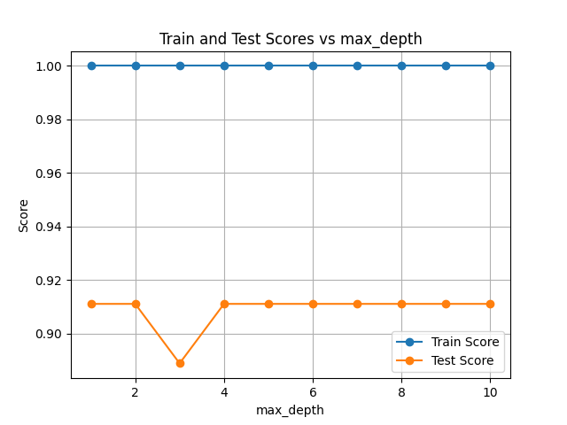
max_depthを1から10で振ってみましたが、特に変化はなくmax_depth=3だけは良くなさそうなことが分かりました。

import numpy as np
import matplotlib.pyplot as plt
from sklearn.datasets import load_iris
from sklearn.model_selection import train_test_split
from sklearn.ensemble import GradientBoostingClassifier

data = load_iris()
X = data.data
y = data.target

X_train, X_test, y_train, y_test = train_test_split(X, y, test_size=0.3, random_state=8)

learning_rates = np.logspace(-3, 0, 10)
train_scores = []
test_scores = []

for lr in learning_rates:
    model = GradientBoostingClassifier(n_estimators=100, learning_rate=lr, max_depth=3, random_state=8)
    model.fit(X_train, y_train)
    
    train_scores.append(model.score(X_train, y_train))
    test_scores.append(model.score(X_test, y_test))

plt.plot(learning_rates, train_scores, label='Train Score', marker='o')
plt.plot(learning_rates, test_scores, label='Test Score', marker='o')
plt.xscale('log')
plt.xlabel('Learning Rate')
plt.ylabel('Score')
plt.title('Train and Test Scores vs Learning Rate')
plt.legend()
plt.grid(True)
plt.show()

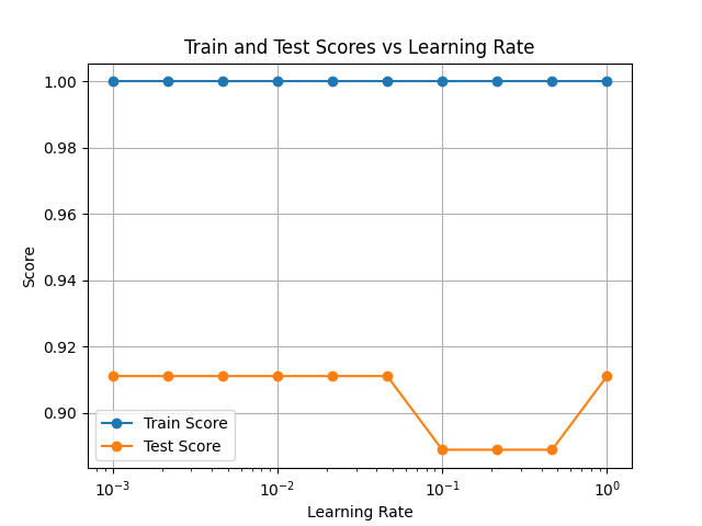
今度はlearning_rateを0.001から1まで10間隔で振ってみました。どうやら最初に選んだmax_depth=3, learning_rate=0.1という組み合わせは一番よくなさそうです。

max_depth=2, learning_rate=0.001に変更した結果が下記です。あやめデータセットのようなシンプルなデータセットは、アンサンブルでは決定木を超えることはありませんでした。

train score: 0.9904761904761905
test score: 0.8888888888888888

■複雑なデータセットで比較してみる

より複雑なscikit-learn標準のデータセットであるdigitsデータセットで学習させてみたいと思います。

●決定木

import numpy as np
import matplotlib.pyplot as plt
from sklearn.datasets import load_digits
from sklearn.model_selection import train_test_split
from sklearn.tree import DecisionTreeClassifier

data = load_digits()
X = data.data
y = data.target

X_train, X_test, y_train, y_test = train_test_split(X, y, test_size=0.3, random_state=8)

max_depths = range(1, 11)
train_scores = []
test_scores = []

for depth in max_depths:
    model = DecisionTreeClassifier(max_depth=depth, random_state=8)
    model.fit(X_train, y_train)
    train_scores.append(model.score(X_train, y_train))
    test_scores.append(model.score(X_test, y_test))

plt.figure(figsize=(10, 6))
plt.plot(max_depths, train_scores, label='Train Score', marker='o')
plt.plot(max_depths, test_scores, label='Test Score', marker='o')
plt.xlabel('Max Depth')
plt.ylabel('Score')
plt.title('Train and Test Scores vs Max Depth')
plt.xticks(max_depths)
plt.legend()
plt.grid()
plt.show()

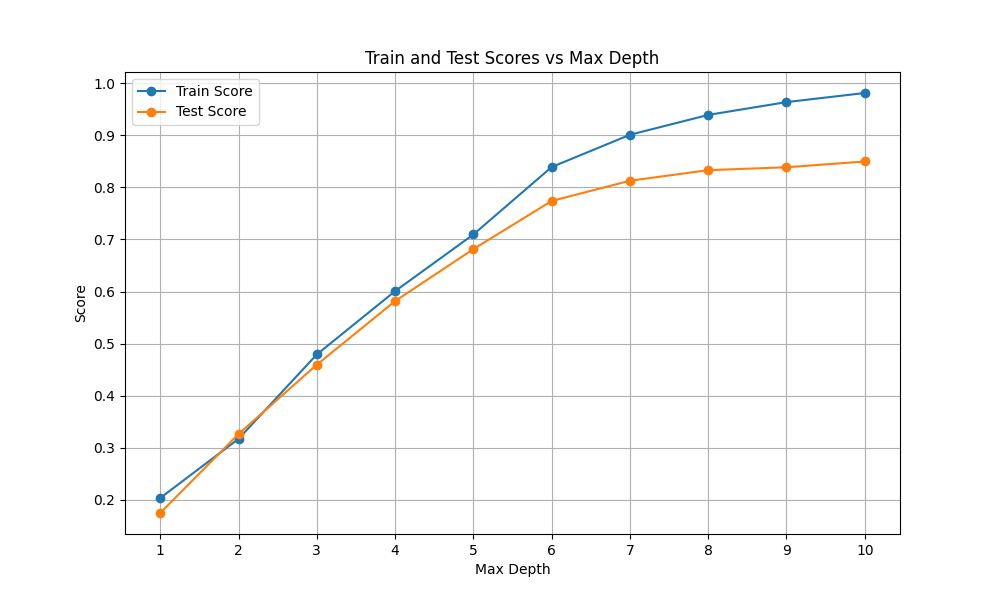
max_depthを1から10の間で振って最適化してみました。どの深さにしてもテストスコア0.9を超えることはなく、それ以前に既に過剰適合の兆候があります。

これ以上の改善は難しそうです。

●ランダムフォレスト

import numpy as np
import matplotlib.pyplot as plt
from sklearn.datasets import load_digits
from sklearn.model_selection import train_test_split
from sklearn.ensemble import RandomForestClassifier

data = load_digits()
X = data.data
y = data.target

X_train, X_test, y_train, y_test = train_test_split(X, y, test_size=0.3, random_state=8)

max_depths = range(1, 11)
train_scores = []
test_scores = []

for depth in max_depths:
    model = RandomForestClassifier(n_estimators=100, max_depth=depth, random_state=8)
    model.fit(X_train, y_train)
    train_scores.append(model.score(X_train, y_train))
    test_scores.append(model.score(X_test, y_test))

plt.figure(figsize=(10, 6))
plt.plot(max_depths, train_scores, label='Train Score', marker='o')
plt.plot(max_depths, test_scores, label='Test Score', marker='o')
plt.xlabel('Max Depth')
plt.ylabel('Score')
plt.title('Train and Test Scores vs Max Depth (Random Forest)')
plt.xticks(max_depths)
plt.legend()
plt.grid()
plt.show()

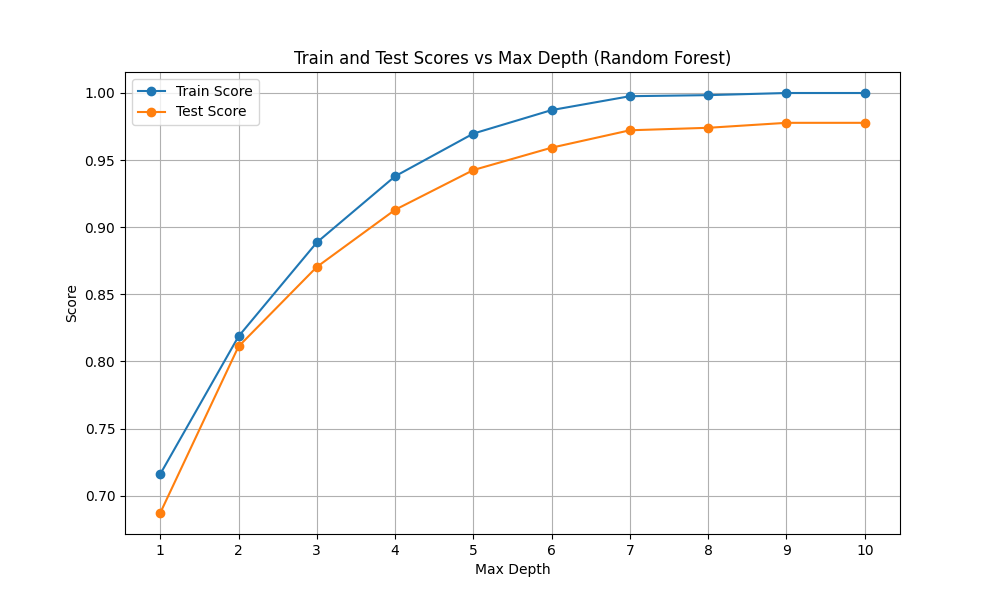
簡単にテストスコア0.95を超えています。また、常にトレーニングスコアの方が高いものの、良い間隔で学習していってます。

デフォルトでこの性能は決定木を圧倒しています。

●勾配ブースティング回帰木

import numpy as np
import matplotlib.pyplot as plt
from sklearn.datasets import load_digits
from sklearn.model_selection import train_test_split
from sklearn.ensemble import GradientBoostingClassifier

data = load_digits()
X = data.data
y = data.target

X_train, X_test, y_train, y_test = train_test_split(X, y, test_size=0.3, random_state=8)

max_depths = range(1, 11)
train_scores = []
test_scores = []

for depth in max_depths:
    model = GradientBoostingClassifier(n_estimators=100, max_depth=depth, learning_rate=0.1, random_state=8)
    model.fit(X_train, y_train)
    train_scores.append(model.score(X_train, y_train))
    test_scores.append(model.score(X_test, y_test))

plt.figure(figsize=(10, 6))
plt.plot(max_depths, train_scores, label='Train Score', marker='o')
plt.plot(max_depths, test_scores, label='Test Score', marker='o')
plt.xlabel('Max Depth')
plt.ylabel('Score')
plt.title('Train and Test Scores vs Max Depth (Gradient Boosting)')
plt.xticks(max_depths)
plt.legend()
plt.grid()
plt.show()

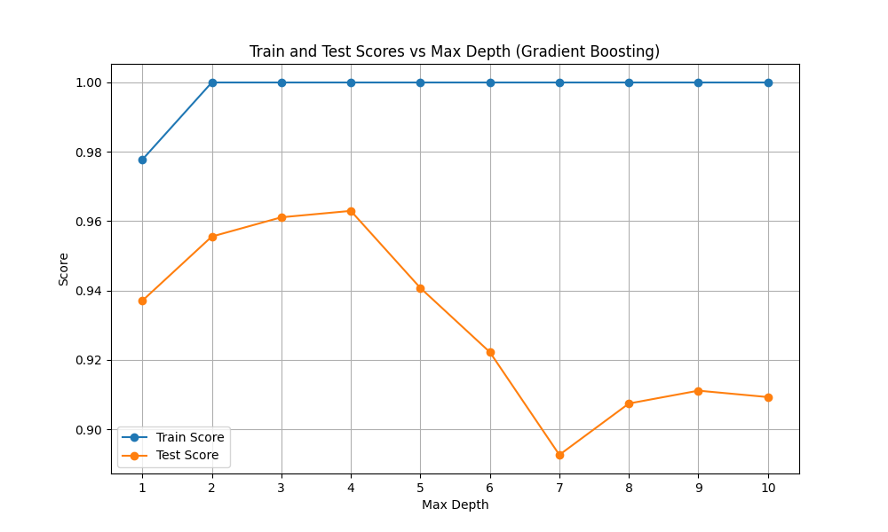
max_depthは1から4程度が良さそうです。

import numpy as np
import matplotlib.pyplot as plt
from sklearn.datasets import load_digits
from sklearn.model_selection import train_test_split
from sklearn.ensemble import GradientBoostingClassifier

data = load_digits()
X = data.data
y = data.target

X_train, X_test, y_train, y_test = train_test_split(X, y, test_size=0.3, random_state=8)

max_depths = range(1, 6)  # 1から5まで
learning_rates = [0.001, 0.01, 0.1, 1]

plt.figure(figsize=(15, 10))

for idx, learning_rate in enumerate(learning_rates):
    train_scores_depth = []
    test_scores_depth = []
    
    for max_depth in max_depths:
        model = GradientBoostingClassifier(n_estimators=100, max_depth=max_depth, learning_rate=learning_rate, random_state=8)
        model.fit(X_train, y_train)
        train_scores_depth.append(model.score(X_train, y_train))
        test_scores_depth.append(model.score(X_test, y_test))
    
    plt.subplot(2, 2, idx + 1)
    plt.plot(max_depths, train_scores_depth, label='Train Score', marker='o')
    plt.plot(max_depths, test_scores_depth, label='Test Score', marker='o')
    plt.xlabel('Max Depth')
    plt.ylabel('Score')
    plt.title(f'Learning Rate = {learning_rate}')
    plt.xticks(max_depths)
    plt.ylim(0, 1)
    plt.legend()
    plt.grid()

plt.tight_layout()
plt.show()

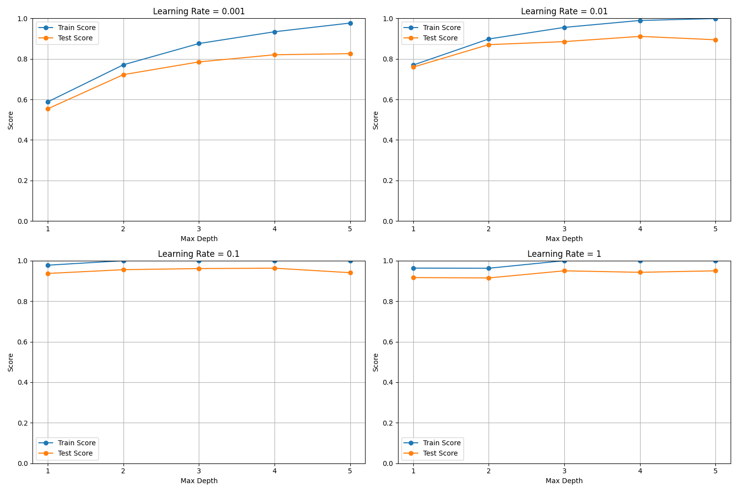
max_depthを1から5まで、learning_rateを0.001から1まで振ってみました。max_depth=2, learning_rate=0.01あたりが良さそうでしょうか。

■おわりに

勾配ブースティング回帰木は使いこなすには中々苦労しそうですが、最適化できればかなりの性能を出せそうです。特に良いトレーニングスコアを維持したままそれを超えそうなテストスコアを出すまでに学習できました。簡単に使うにはランダムフォレストもかなり良い選択で、前処理もなくほぼ無調整で十分なスコアだったかと思います。

これらのアンサンブル法を使うまでもないデータセットに対してはシンプルな決定木1本で十分機能することも理解できました。

どのモデルも総じて速く、挙動が理解しやすかったです。（アンサンブルであってもパラメータ自体は単純。）決定木が好まれる理由が良く分かりました。

■参考文献

1. Andreas C. Muller, Sarah Guido. Pythonではじめる機械学習. 中田 秀基 訳. オライリー・ジャパン. 2017. 392p.
2. ChatGPT. 4o mini. OpenAI. 2024. https://chatgpt.com/
3. API Reference. scikit-learn.org. https://scikit-learn.org/stable/api/index.html
4. 決定木分析（デシジョン・ツリー）とは. ibm.com. https://www.ibm.com/jp-ja/topics/decision-trees